Qualified
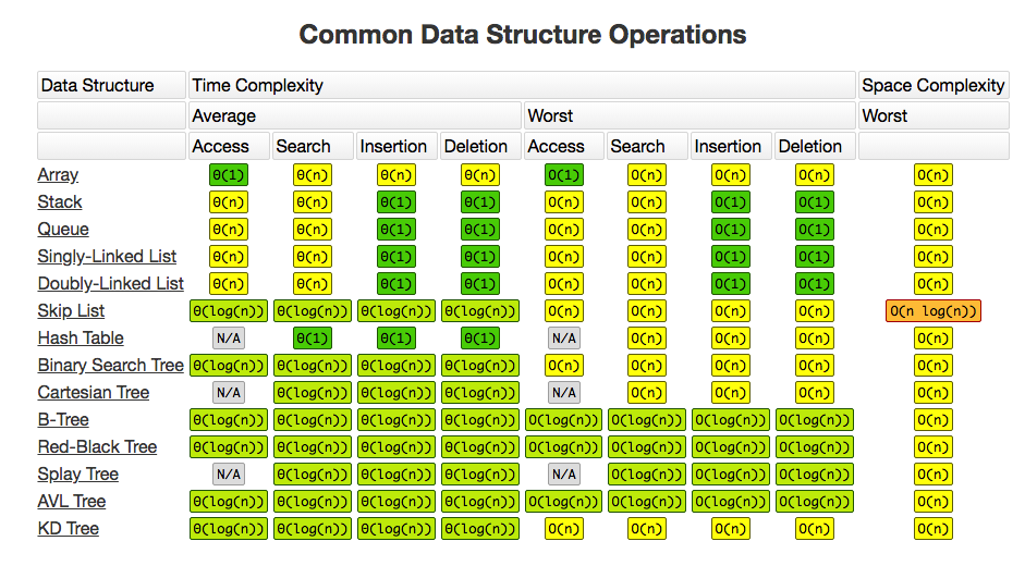
Algorithms complexity (understanding, big O notation, complexity of common algorithms)
Stack, queue, linked list(construction, understanding, usage)
Algorithms complexity (understanding, big O notation, complexity of common algorithms)
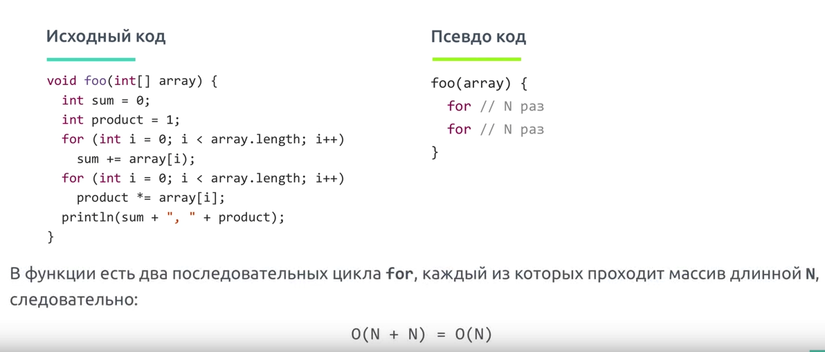
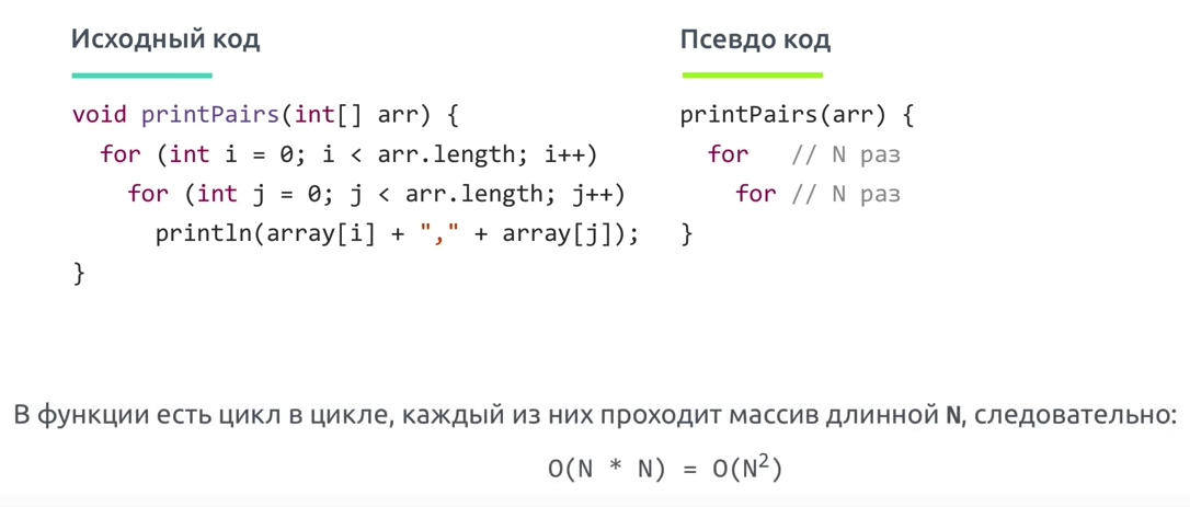
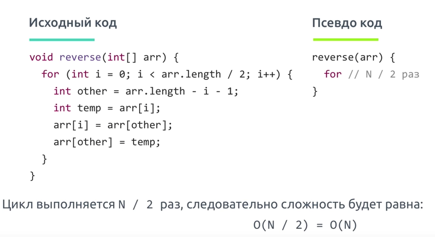
Big O
Big O показывает верхнюю границу зависимости между входными параметрами функции и количеством операций, которые выполнит процессор
Big O
Big o is simplified analysis of an algorithm's efficiency
- complexity in terms ofinput size, n
- machine-independent
- basic computer steps
- time & space
Types of measurements
- worst-case
- best-case
- average-case
оценка по времени, оценка по памяти
Big O notation is the language we use for talking about how long an algorithm takes to run. It's how we compare the efficiency of different approaches to a problem.
It's like math except it's an awesome, not-boring kind of math where you get to wave your hands through the details and just focus on what's basically happening.
With big O notation we express the runtime in terms of—brace yourself—how quickly it grows relative to the input, as the input gets arbitrarily large.
Let's break that down:
- how quickly the runtime grows — it's hard to pin down the exact runtime of an algorithm. It depends on the speed of the processor, what else the computer is running, etc. So instead of talking about the runtime directly, we use big O notation to talk about how quickly the runtime grows.
- relative to the input - if we were measuring our runtime directly, we could express our speed in seconds. Since we're measuring how quickly our runtime grows, we need to express our speed in terms of...something else. With Big O notation, we use the size of the input, which we call "n." So we can say things like the runtime grows "on the order of the size of the input" (O(n)) or "on the order of the square of the size of the input" (O(n2))
- as the input gets arbitrarily large - our algorithm may have steps that seem expensive when nn is small but are eclipsed eventually by other steps as nn gets huge. For big O analysis, we care most about the stuff that grows fastest as the input grows, because everything else is quickly eclipsed as nn gets very large. (If you know what an asymptote is, you might see why "big O analysis" is sometimes called "asymptotic analysis.")
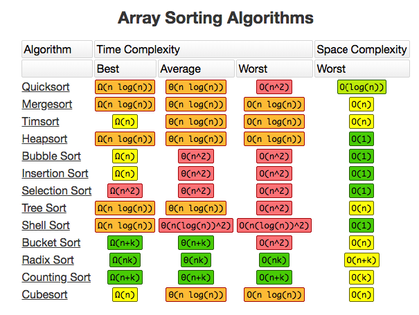
Array sorting methods(bubble sort, quick sort, merge sort)
Bubble sort
TIP
Bubble sort is a simple sorting algorithm. This sorting algorithm is comparison-based algorithm in which each pair of adjacent elements is compared and the elements are swapped if they are not in order. This algorithm is not suitable for large data sets as its average and worst case complexity are of Ο(n2) where n is the number of items.
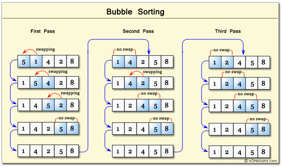
If the given array has to be sorted in ascending order, then bubble sort will start by comparing the first element of the array with the second element, if the first element is greater than the second element, it will swap both the elements, and then move on to compare the second and the third element, and so on.
If we have total n elements, then we need to repeat this process for n-1 times.
It is known as bubble sort, because with every complete iteration the largest element in the given array, bubbles up towards the last place or the highest index, just like a water bubble rises up to the water surface.
Sorting takes place by stepping through all the elements one-by-one and comparing it with the adjacent element and swapping them if required.
Quick sort
Quick sort
QuickSort is a Divide and Conquer algorithm. It picks an element as pivot and partitions the given array around the picked pivot. There are many different versions of quickSort that pick pivot in different ways.
Основная идея заключается в том, чтобы найти опорный элемент в массиве для сравнения с остальными частями, затем сдвигать элементы так, чтобы все части перед опорным элементом были меньше его, а все элементы после опорного были больше его. После этого рекурсивно выполнить ту же операцию на элементы до и после опорного.
- Always pick first element as pivot.
- Always pick last element as pivot (implemented below)
- Pick a random element as pivot.
- Pick median as pivot.
The key process in quickSort is partition(). Target of partitions is, given an array and an element x of array as pivot, put x at its correct position in sorted array and put all smaller elements (smaller than x) before x, and put all greater elements (greater than x) after x. All this should be done in linear time.
Pseudo Code for recursive QuickSort function
/* low  --> Starting index,  high  --> Ending index */
quickSort(arr[], low, high)
{
    if (low < high)
    {
        /* pi is partitioning index, arr[pi] is now
           at right place */
        pi = partition(arr, low, high);

        quickSort(arr, low, pi - 1);  // Before pi
        quickSort(arr, pi + 1, high); // After pi
    }
}
Основные шаги для разделения массива:
- Найти опорный элемент в массиве. Этот элемент — основа для сравнения за одни проход.
- Установить указатель (левый указатель) с первого элемента в массиве.
- Установить указатель (правый указатель) с последнего элемента в массиве.
- Пока значение левого указателя в массиве меньше, чем значение опорного элемента, сдвигать левый указатель вправо (добавить 1). Продолжить пока значение левого указателя не станет большим или равным опорному.
- Пока значение правого указателя в массиве больше, чем значение опорного элемента, сдвигать правый указатель влево (вычитать 1). Продолжать пока значение правого указателя не станет меньшим или равным значению разделителя.
- Если левый указатель меньше или равен правому указателю, поменять значения в этих местах в массиве.
- Сдвинуть левый указатель вправо на одну позицию и правый указатель на одну позицию влево.
- Если левый указатель и правый указатель не встретятся, перейти к шагу 1.
merge sort
- Разбитие массива на мелкие части одинакового размера. Рекурсивно массив разбивается пока у нас не будет отдельных элементов
- Сливаем части “соседних массивов” в один с сортировкой. Опять же, сортировка проходит достачтоно интересно: так как мы сливаем уже сортированные массивы — в результате хотелось бы получить сортированный массив. Итак, допустим у нас есть два массива:
2.1 Указатели указывают на первый элемент обоих массивов. Выбирается наименьший из них
2.2 В массиве в котором было наименьшее число — указатель переноситься на следующий элемент. Повторяем пункт 2.1
2.3 Если в одном из массивов закончились элементы — переносим элементы другого массива в наш отсортированный массив ( слив остатков )
- Повторяем пока подмасивы не закончатся
Tree structure(construction, traversal)
Trees: Unlike Arrays, Linked Lists, Stack and queues, which are linear data structures, trees are hierarchical data structures. Tree Vocabulary: The topmost node is called root of the tree. The elements that are directly under an element are called its children. The element directly above something is called its parent. For example, ‘a’ is a child of ‘f’, and ‘f’ is the parent of ‘a’. Finally, elements with no children are called leaves.
Tree is a hierarchical data structure. Main uses of trees include maintaining hierarchical data, providing moderate access and insert/delete operations. Binary trees are special cases of tree where every node has at most two children.
      tree
      ----
       j    <-- root
     /   \
    f      k
  /   \      \
 a     h      z    <-- leaves
- One reason to use trees might be because you want to store information that naturally forms a hierarchy. For example, the file system on a computer:
file system
-----------
     /    <-- root
  /      \
...       home
      /          \
   ugrad        course
    /       /      |     \
  ...      cs101  cs112  cs113
- Trees (with some ordering e.g., BST) provide moderate access/search (quicker than Linked List and slower than arrays).
- Trees provide moderate insertion/deletion (quicker than Arrays and slower than Unordered Linked Lists).
- Like Linked Lists and unlike Arrays, Trees don’t have an upper limit on number of nodes as nodes are linked using pointers.
Main applications of trees include:
- Manipulate hierarchical data.
- Make information easy to search (see tree traversal).
- Manipulate sorted lists of data.
- As a workflow for compositing digital images for visual effects.
- Router algorithms
- Form of a multi-stage decision-making (see business chess).
Binary Tree: A tree whose elements have at most 2 children is called a binary tree. Since each element in a binary tree can have only 2 children, we typically name them the left and right child.
Properties
- The maximum number of nodes at level ‘l’ of a binary tree is 2l-1.
- Maximum number of nodes in a binary tree of height ‘h’ is 2h – 1.
- In a Binary Tree with N nodes, minimum possible height or minimum number of levels is Log2(N+1)
- In Binary tree where every node has 0 or 2 children, number of leaf nodes is always one more than nodes with two children.
Бинарное дерево — это иерархическая структура данных, в которой каждый узел имеет значение (оно же является в данном случае и ключом) и ссылки на левого и правого потомка. Узел, находящийся на самом верхнем уровне (не являющийся чьим либо потомком) называется корнем. Узлы, не имеющие потомков (оба потомка которых равны NULL) называются листьями.
Бинарное дерево поиска — это бинарное дерево, обладающее дополнительными свойствами: значение левого потомка меньше значения родителя, а значение правого потомка больше значения родителя для каждого узла дерева. То есть, данные в бинарном дереве поиска хранятся в отсортированном виде. При каждой операции вставки нового или удаления существующего узла отсортированный порядок дерева сохраняется. При поиске элемента сравнивается искомое значение с корнем. Если искомое больше корня, то поиск продолжается в правом потомке корня, если меньше, то в левом, если равно, то значение найдено и поиск прекращается.
Поиск минимального значения невероятно прост — это всегда самый левый узел, то есть мы пробегаем по всем потомкам, если у потомка есть левый лист, значит бежим по его потомкам. Как только мы видим, что потомков нет — вуаля, у нас самое маленькое значение
Тоже самое с самым большим значением — оно всегда самое правое
Поиск элемента тоже очень прост:
- Как обычно начинаем с корневого элемента.
- Проверяем или даный элемент — тот который нам нужен. Если да — возвращаем
- и нет: смотрим или он больше даного, или меньше. Идем к соответствующему листу
- Если листов нет — элемента нет. Если есть — повторяем пункт 2.
Traversals
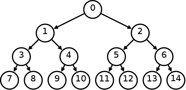
Unlike linear data structures (Array, Linked List, Queues, Stacks, etc) which have only one logical way to traverse them, trees can be traversed in different ways. Following are the generally used ways for traversing trees.

Depth First Traversals:
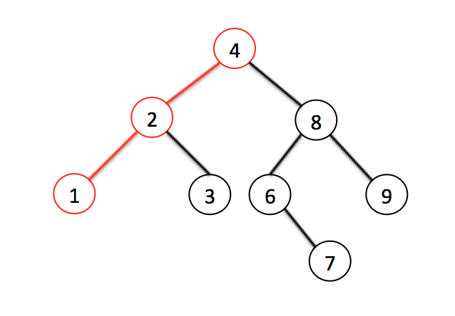
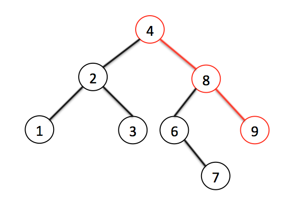
- (a) Inorder (Left, Root, Right) : 4 2 5 1 3
- (b) Preorder (Root, Left, Right) : 1 2 4 5 3
- (c) Postorder (Left, Right, Root) : 4 5 2 3 1
Breadth First or Level Order Traversal : 1 2 3 4 5
Inorder Traversal (Practice):
Algorithm Inorder(tree)
   1. Traverse the left subtree, i.e., call Inorder(left-subtree)
   2. Visit the root.
   3. Traverse the right subtree, i.e., call Inorder(right-subtree)
In case of binary search trees (BST), Inorder traversal gives nodes in non-decreasing order. To get nodes of BST in non-increasing order, a variation of Inorder traversal where Inorder traversal s reversed can be used.
Example: Inorder traversal for the above-given figure is 4 2 5 1 3.
Preorder Traversal (Practice):
Algorithm Preorder(tree)
   1. Visit the root.
   2. Traverse the left subtree, i.e., call Preorder(left-subtree)
   3. Traverse the right subtree, i.e., call Preorder(right-subtree)
Preorder traversal is used to create a copy of the tree. Preorder traversal is also used to get prefix expression on of an expression tree. Example: Preorder traversal for the above given figure is 1 2 4 5 3.
Postorder Traversal (Practice):
Algorithm Postorder(tree)
   1. Traverse the left subtree, i.e., call Postorder(left-subtree)
   2. Traverse the right subtree, i.e., call Postorder(right-subtree)
   3. Visit the root.
Postorder traversal is used to delete the tree. Please see the question for deletion of tree for details. Postorder traversal is also useful to get the postfix expression of an expression tree.
Example: Postorder traversal for the above given figure is 4 5 2 3 1.
Binary search algorithm
Binary Search: Search a sorted array by repeatedly dividing the search interval in half. Begin with an interval covering the whole array. If the value of the search key is less than the item in the middle of the interval, narrow the interval to the lower half. Otherwise narrow it to the upper half. Repeatedly check until the value is found or the interval is empty.
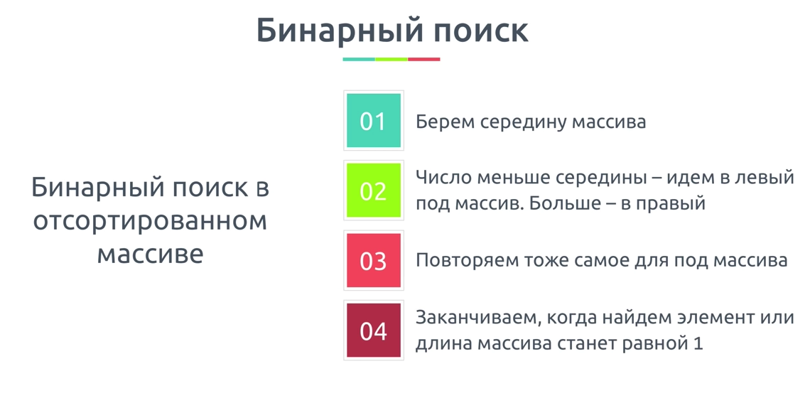
We basically ignore half of the elements just after one comparison.
- Compare x with the middle element.
- *If x matches with middle element, we return the mid index.
- Else If x is greater than the mid element, then x can only lie in right half subarray after the mid element. So we recur for right half.
- Else (x is smaller) recur for the left half.
Hash table(creating, collisions)
Hash Table is a data structure which stores data in an associative manner. In a hash table, data is stored in an array format, where each data value has its own unique index value. Access of data becomes very fast if we know the index of the desired data.
Thus, it becomes a data structure in which insertion and search operations are very fast irrespective of the size of the data. Hash Table uses an array as a storage medium and uses hash technique to generate an index where an element is to be inserted or is to be located from.
Hashing is a technique that is used to uniquely identify a specific object from a group of similar objects. Some examples of how hashing is used in our lives include:
- In universities, each student is assigned a unique roll number that can be used to retrieve information about them.
- In libraries, each book is assigned a unique number that can be used to determine information about the book, such as its exact position in the library or the users it has been issued to etc.
In both these examples the students and books were hashed to a unique number.
Assume that you have an object and you want to assign a key to it to make searching easy. To store the key/value pair, you can use a simple array like a data structure where keys (integers) can be used directly as an index to store values. However, in cases where the keys are large and cannot be used directly as an index, you should use hashing.
In hashing, large keys are converted into small keys by using hash functions. The values are then stored in a data structure called hash table. The idea of hashing is to distribute entries (key/value pairs) uniformly across an array. Each element is assigned a key (converted key). By using that key you can access the element in O(1) time. Using the key, the algorithm (hash function) computes an index that suggests where an entry can be found or inserted.
Hashing is implemented in two steps:
- An element is converted into an integer by using a hash function. This element can be used as an index to store the original element, which falls into the hash table.
- The element is stored in the hash table where it can be quickly retrieved using hashed key.
hash = hashfunc(key)
index = hash % array_size
In this method, the hash is independent of the array size and it is then reduced to an index (a number between 0 and array_size − 1) by using the modulo operator (%).
Hash function
A hash function is any function that can be used to map a data set of an arbitrary size to a data set of a fixed size, which falls into the hash table. The values returned by a hash function are called hash values, hash codes, hash sums, or simply hashes.
To achieve a good hashing mechanism, It is important to have a good hash function with the following basic requirements:
- Easy to compute: It should be easy to compute and must not become an algorithm in itself.
- Uniform distribution: It should provide a uniform distribution across the hash table and should not result in clustering.
- Less collisions: Collisions occur when pairs of elements are mapped to the same hash value. These should be avoided.
Note
Irrespective of how good a hash function is, collisions are bound to occur. Therefore, to maintain the performance of a hash table, it is important to manage collisions through various collision resolution techniques.
:::tipHash table A hash table is a data structure that is used to store keys/value pairs. It uses a hash function to compute an index into an array in which an element will be inserted or searched. By using a good hash function, hashing can work well. Under reasonable assumptions, the average time required to search for an element in a hash table is O(1). :::
Collisions
What is Collision?
Since a hash function gets us a small number for a key which is a big integer or string, there is a possibility that two keys result in the same value. The situation where a newly inserted key maps to an already occupied slot in the hash table is called collision and must be handled using some collision handling technique.
What are the chances of collisions with large table?
Collisions are very likely even if we have big table to store keys. An important observation is Birthday Paradox. With only 23 persons, the probability that two people have the same birthday is 50%.
How to handle Collisions?
There are mainly two methods to handle collision:
- Separate Chaining
- Open Addressing
Separate Chaining
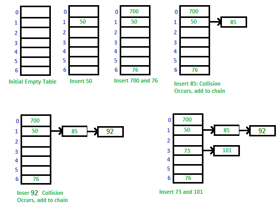
The idea is to make each cell of hash table point to a linked list of records that have same hash function value.
Let us consider a simple hash function as “key mod 7” and sequence of keys as 50, 700, 76, 85, 92, 73, 101.
Advantages
- Simple to implement.
- Hash table never fills up, we can always add more elements to the chain.
- Less sensitive to the hash function or load factors.
- It is mostly used when it is unknown how many and how frequently keys may be inserted or deleted.
Disadvantages
- Cache performance of chaining is not good as keys are stored using a linked list. Open addressing provides better cache performance as everything is stored in the same table.
- Wastage of Space (Some Parts of hash table are never used)
- If the chain becomes long, then search time can become O(n) in the worst case.
- Uses extra space for links.
As you might be knowing that hash table data structure works on key value pairing. The idea behind using of Hash table is it would work with O(1) time complexity for insertion, deletion and search operations in Hash Table for any given value. O(1) time complexity can be achieved if we have a key for each value. Calculation of key for a given value is done by hash functions. eg.- If we want to do some operations on characters used in a string we can use ASCII value of characters as key. This way each character (value) would be mapped to different ascii (key). Suppose if you also want to keep track of number of occurrences of characters or you want to store repeated characters also in hash table than collision will occur. Because repeated characters will collide with already stored characters in has table for the keys. In this example it may not look a big deal as characters are identical but in some other cases it would affect the desired result of O(1). In worst case operations can cost O(n). So collisions occur when more than one value link to single key in hash table. We can add values in linked list for that key in such cases.
To avoid the collision hash function should be properly picked. It can also depend on the size of hash table. If you have wide range of inputs its quite possible that for a particular set of input you will always get worst case O(n) time complexity. To overcome that we can have a set of hash functions and we can randomly pic a hash function on execution. This would avoid the situations where a given input always leads to worst case performance. There are some other techniques also like Open Addressing. You can refer Cormen Book to know more about it.
Stack, queue, linked list(construction, understanding, usage)
LinkedList
LinkedList
Linked List is a very commonly used linear data structure which consists of group of nodes in a sequence. Each node holds its own data and the address of the next node hence forming a chain like structure.
Linked Lists are used to create trees and graphs.

Advantages of Linked Lists
- They are a dynamic in nature which allocates the memory when required.
- Insertion and deletion operations can be easily implemented.
- Stacks and queues can be easily executed.
- Linked List reduces the access time.
Disadvantages of Linked Lists
- The memory is wasted as pointers require extra memory for storage.
- No element can be accessed randomly; it has to access each node sequentially.
- Reverse Traversing is difficult in linked list.
Applications of Linked Lists
- Linked lists are used to implement stacks, queues, graphs, etc.
- Linked lists let you insert elements at the beginning and end of the list.
- In Linked Lists we don't need to know the size in advance.
There are 3 different implementations of Linked List available, they are:
- Singly Linked List
- Doubly Linked List
- Circular Linked List
Singly Linked List
Singly linked lists contain nodes which have a data part as well as an address part i.e. next, which points to the next node in the sequence of nodes.
The operations we can perform on singly linked lists are insertion, deletion and traversal.

Doubly Linked List
In a doubly linked list, each node contains a data part and two addresses, one for the previous node and one for the next node.

Circular Linked List
In circular linked list the last node of the list holds the address of the first node hence forming a circular chain.

Difference between Array and Linked List
Both Linked List and Array are used to store linear data of similar type, but an array consumes contiguous memory locations allocated at compile time, i.e. at the time of declaration of array, while for a linked list, memory is assigned as and when data is added to it, which means at runtime.
This is the basic and the most important difference between a linked list and an array. In the section below, we will discuss this in details along with highlighting other differences.
- *Linked List vs. Array Array is a datatype which is widely implemented as a default type, in almost all the modern programming languages, and is used to store data of similar type.
But there are many usecases, like the one where we don't know the quantity of data to be stored, for which advanced data structures are required, and one such data structure is linked list.
| ARRAY | LINKED LIST |
|---|---|
| Array is a collection of elements of similar data type. | Linked List is an ordered collection of elements of same type, which are connected to each other using pointers. |
| Array supports Random Access, which means elements can be accessed directly using their index, like arr[0] for 1st element, arr[6] for 7th element etc. Hence, accessing elements in an array is fast with a constant time complexity of O(1). | Linked List supports Sequential Access, which means to access any element/node in a linked list, we have to sequentially traverse the complete linked list, upto that element. To access nth element of a linked list, time complexity is O(n). |
| In an array, elements are stored in contiguous memory location or consecutive manner in the memory. | In a linked list, new elements can be stored anywhere in the memory. Address of the memory location allocated to the new element is stored in the previous node of linked list, hence formaing a link between the two nodes/elements. |
| In array, Insertion and Deletion operation takes more time, as the memory locations are consecutive and fixed. | In case of linked list, a new element is stored at the first free and available memory location, with only a single overhead step of storing the address of memory location in the previous node of linked list. Insertion and Deletion operations are fast in linked list. |
| Memory is allocated as soon as the array is declared, at compile time. It's also known as Static Memory Allocation. | Memory is allocated at runtime, as and when a new node is added. It's also known as Dynamic Memory Allocation. |
| In array, each element is independent and can be accessed using it's index value. | In case of a linked list, each node/element points to the next, previous, or maybe both nodes. |
| Array can single dimensional, two dimensional or multidimensional | Linked list can be Linear(Singly), Doubly or Circular linked list. |
| Size of the array must be specified at time of array decalaration. | Size of a Linked list is variable. It grows at runtime, as more nodes are added to it. |
| Array gets memory allocated in the Stack section. | Whereas, linked list gets memory allocated in Heap section. |
Below we have a pictorial representation showing how consecutive memory locations are allocated for array, while in case of linked list random memory locations are assigned to nodes, but each node is connected to its next node using pointer.

- Why we need pointers in Linked List? In case of array, memory is allocated in contiguous manner, hence array elements get stored in consecutive memory locations. So when you have to access any array element, all we have to do is use the array index, for example arr[4] will directly access the 5th memory location, returning the data stored there.
But in case of linked list, data elements are allocated memory at runtime, hence the memory location can be anywhere. Therefore to be able to access every node of the linked list, address of every node is stored in the previous node, hence forming a link between every node.
We need this additional pointer because without it, the data stored at random memory locations will be lost. We need to store somewhere all the memory locations where elements are getting stored.
Yes, this requires an additional memory space with each node, which means an additional space of O(n) for every n node linked list.
Stack
Stack is an abstract data type with a bounded(predefined) capacity. It is a simple data structure that allows adding and removing elements in a particular order. Every time an element is added, it goes on the top of the stack and the only element that can be removed is the element that is at the top of the stack, just like a pile of objects.

Basic features of Stack
- Stack is an ordered list of similar data type.
- Stack is a LIFO(Last in First out) structure or we can say FILO(First in Last out).
- push() function is used to insert new elements into the Stack and pop() function is used to remove an element from the stack. Both insertion and removal are allowed at only one end of Stack called Top.
- Stack is said to be in Overflow state when it is completely full and is said to be in Underflow state if it is completely empty.
Applications of Stack
The simplest application of a stack is to reverse a word. You push a given word to stack - letter by letter - and then pop letters from the stack. There are other uses also like:
- Parsing
- Expression Conversion(Infix to Postfix, Postfix to Prefix etc)
Implementation of Stack Data Structure
Stack can be easily implemented using an Array or a Linked List. Arrays are quick, but are limited in size and Linked List requires overhead to allocate, link, unlink, and deallocate, but is not limited in size. Here we will implement Stack using array.

Algorithm for PUSH operation
- Check if the stack is full or not.
- If the stack is full, then print error of overflow and exit the program.
- If the stack is not full, then increment the top and add the element.
Algorithm for POP operation
- Check if the stack is empty or not.
- If the stack is empty, then print error of underflow and exit the program.
- If the stack is not empty, then print the element at the top and decrement the top.
Analysis of Stack Operations
Below mentioned are the time complexities for various operations that can be performed on the Stack data structure.
- Push Operation : O(1)
- Pop Operation : O(1)
- Top Operation : O(1)
- Search Operation : O(n)
The time complexities for push() and pop() functions are O(1) because we always have to insert or remove the data from the top of the stack, which is a one step process.
Queue
Queue is an abstract data type or a linear data structure, just like stack data structure, in which the first element is inserted from one end called the REAR(also called tail), and the removal of existing element takes place from the other end called as FRONT(also called head).
This makes queue as FIFO(First in First Out) data structure, which means that element inserted first will be removed first.
Which is exactly how queue system works in real world. If you go to a ticket counter to buy movie tickets, and are first in the queue, then you will be the first one to get the tickets. Right? Same is the case with Queue data structure. Data inserted first, will leave the queue first.
The process to add an element into queue is called Enqueue and the process of removal of an element from queue is called Dequeue.

Basic features of Queue
- Like stack, queue is also an ordered list of elements of similar data types.
- Queue is a FIFO( First in First Out ) structure.
- Once a new element is inserted into the Queue, all the elements inserted before the new element in the queue must be removed, to remove the new element.
- peek() function is oftenly used to return the value of first element without dequeuing it.
Applications of Queue
Queue, as the name suggests is used whenever we need to manage any group of objects in an order in which the first one coming in, also gets out first while the others wait for their turn, like in the following scenarios:
- Serving requests on a single shared resource, like a printer, CPU task scheduling etc.
- In real life scenario, Call Center phone systems uses Queues to hold people calling them in an order, until a service representative is free.
- Handling of interrupts in real-time systems. The interrupts are handled in the same order as they arrive i.e First come first served.
Implementation of Queue Data Structure
Queue can be implemented using an Array, Stack or Linked List. The easiest way of implementing a queue is by using an Array.
Initially the head(FRONT) and the tail(REAR) of the queue points at the first index of the array (starting the index of array from 0). As we add elements to the queue, the tail keeps on moving ahead, always pointing to the position where the next element will be inserted, while the head remains at the first index.
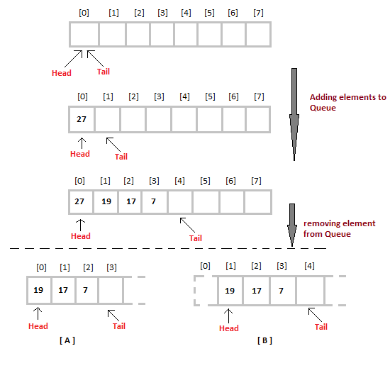
When we remove an element from Queue, we can follow two possible approaches (mentioned [A] and [B] in above diagram). In [A] approach, we remove the element at head position, and then one by one shift all the other elements in forward position.
In approach [B] we remove the element from head position and then move head to the next position.
In approach [A] there is an overhead of shifting the elements one position forward every time we remove the first element.
In approach [B] there is no such overhead, but whenever we move head one position ahead, after removal of first element, the size on Queue is reduced by one space each time.
Algorithm for ENQUEUE operation
- Check if the queue is full or not.
- If the queue is full, then print overflow error and exit the program.
- If the queue is not full, then increment the tail and add the element.
Algorithm for DEQUEUE operation
- Check if the queue is empty or not.
- If the queue is empty, then print underflow error and exit the program.
- If the queue is not empty, then print the element at the head and increment the head.
Complexity Analysis of Queue Operations
Just like Stack, in case of a Queue too, we know exactly, on which position new element will be added and from where an element will be removed, hence both these operations requires a single step.
- Enqueue: O(1)
- Dequeue: O(1)
- Size: O(1)