# Competent

• Cone of Uncertainty
• Source of Estimation Errors
• Diseconomies of Scale
• Count, Compute, Judge techniques
• Delphi method
• Challenges with Estimating Size
• Challenges with Estimating Effort
• Challenges with Estimating Schedule
• Story based scope definition: scoping project, release planning
• Documenting and presenting estimation results
• PERT analysis

---

# Cone of Uncertainty

Software development consists of making literally thousands of decisions about all the feature-related issues described in the previous section. Uncertainty in a software estimate results from uncertainty in how the decisions will be resolved. As you make a greater percentage of those decisions, you reduce the estimation uncertainty.

As a result of this process of resolving decisions, researchers have found that project estimates are subject to predictable amounts of uncertainty at various stages. The Cone of Uncertainty shows how estimates become more accurate as a project progresses. (The following discussion initially describes a sequential development approach for ease of explanation).

The horizontal axis contains common project milestones, such as Initial Concept, Approved Product Definition, Requirements Complete, and so on. Because of its origins, this terminology sounds somewhat product-oriented. "Product Definition" just refers to the agreed-upon vision for the software, or the software concept, and applies equally to Web services, internal business systems, and most other kinds of software projects.

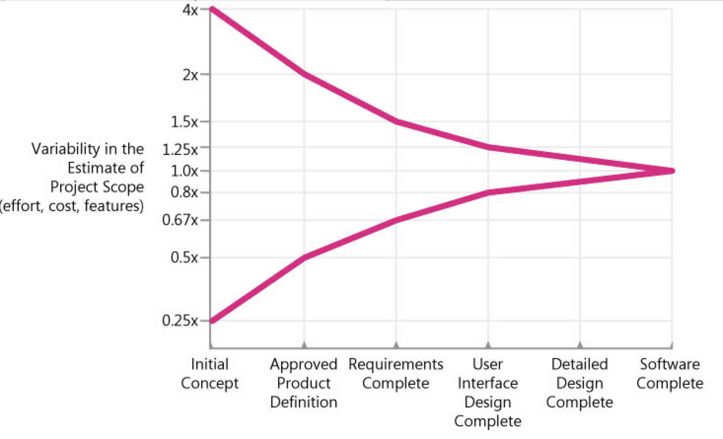
The vertical axis contains the degree of error that has been found in estimates created by skilled estimators at various points in the project. The estimates could be for how much a particular feature set will cost and how much effort will be required to deliver that feature set, or it could be for how many features can be delivered for a particular amount of effort or schedule.

As you can see from the graph, estimates created very early in the project are subject to a high degree of error. Estimates created at Initial Concept time can be inaccurate by a factor of 4x on the high side or 4x on the low side (also expressed as 0.25x, which is just 1 divided by 4). The total range from high estimate to low estimate is 4x divided by 0.25x, or 16x!

One question that managers and customers ask is, "If I give you another week to work on your estimate, can you refine it so that it contains less uncertainty?" That's a reasonable request, but unfortunately it's not possible to deliver on that request. Research by Luiz Laranjeira suggests that the accuracy of the software estimate depends on the level of refinement of the software's definition (Laranjeira 1990). The more refined the definition, the more accurate the estimate. The reason the estimate contains variability is that the software project itself contains variability. The only way to reduce the variability in the estimate is to reduce the variability in the project.

One misleading implication of this common depiction of the Cone of Uncertainty is that it looks like the Cone takes forever to narrow—as if you can't have very good estimation accuracy until you're nearly done with the project. Fortunately, that impression is created because the milestones on the horizontal axis are equally spaced, and we naturally assume that the horizontal axis is calendar time.

An important—and difficult—concept is that the Cone of Uncertainty represents the best-case accuracy that is possible to have in software estimates at different points in a project. The Cone represents the error in estimates created by skilled estimators. It's easily possible to do worse. It isn't possible to be more accurate; it's only possible to be more lucky.

---

# Source of Estimation Errors

The Cone of Uncertainty represents uncertainty that is inherent even in well-run projects. Additional variability can arise from poorly run projects—that is, from avoidable project chaos.

• Requirements that weren't investigated very well in the first place
• Lack of end-user involvement in requirements validation
• Poor designs that lead to numerous errors in the code
• Poor coding practices that give rise to extensive bug fixing
• Inexperienced personnel
• Incomplete or unskilled project planning
• Prima donna team members
• Abandoning planning under pressure
• Developer gold-plating
• Lack of automated source code contro
• Unstable Requirements
• Omitted Activities

One of the most common sources of estimation error is forgetting to include necessary tasks in the project estimates (Lederer and Prasad 1992, Coombs 2003). Researchers have found that this phenomenon applies both at the project planning level and at the individual developer level. One study found that developers tended to estimate pretty accurately the work they remembered to estimate, but they tended to overlook 20% to 30% of the necessary tasks, which led to a 20 to 30% estimation error (van Genuchten 1991).

Omitted work falls into three general categories: missing requirements, missing software-development activities, and missing non-software-development activities.

# Functional and Nonfunctional Requirements Commonly Missing from Software Estimates

• Setup/installation program
• Interfaces with external systems
• Help system
• Glue code needed to use third-party or open-source software

# Software-Development Activities Commonly Missing from Software Estimates

• Ramp-up time for new team members
• Mentoring of new team members
• Management coordination/manager meetings
• Cutover/deployment
• Data conversion
• Installation
• Customization
• Requirements clarifications
• Review of technical documentation
• Demonstrating software to customers or users

# Non-Software-Development Activities Commonly Missing from Software Estimates

• Vacations
• Company meetings
• Holidays
• Department meetings
• Sick days
• Setting up new workstations
• Training
• Installing new versions of tools on workstations
• Weekends
• Troubleshooting hardware and software problems
• Unfounded Optimism
• Subjectivity and Bias
• Unwarranted Precision
• Unfamiliar business area
• Unfamiliar technology area
• Incorrect conversion from estimated time to project time (for example, assuming the project team will focus on the project eight hours per day, five days per week)
• Misunderstanding of statistical concepts (especially adding together a set of "best case" estimates or a set of "worst case" estimates)
• Budgeting processes that undermine effective estimation (especially those that require final budget approval in the wide part of the Cone of Uncertainty)
• Having an accurate size estimate, but introducing errors when converting the size estimate to an effort estimate
• Having accurate size and effort estimates, but introducing errors when converting those to a schedule estimate
• Overstated savings from new development tools or methods

---

# Diseconomies of Scale

People naturally assume that a system that is 10 times as large as another system will require something like 10 times as much effort to build. But the effort for a 1,000,000-LOC system is more than 10 times as large as the effort for a 100,000-LOC system, as is the effort for a 100,000-LOC system compared to the effort for a 10,000-LOC system. The basic issue is that, in software, larger projects require coordination among larger groups of people, which requires more communication (Brooks 1995). As project size increases, the number of communication paths among different people increases as a squared function of the number of people on the project.

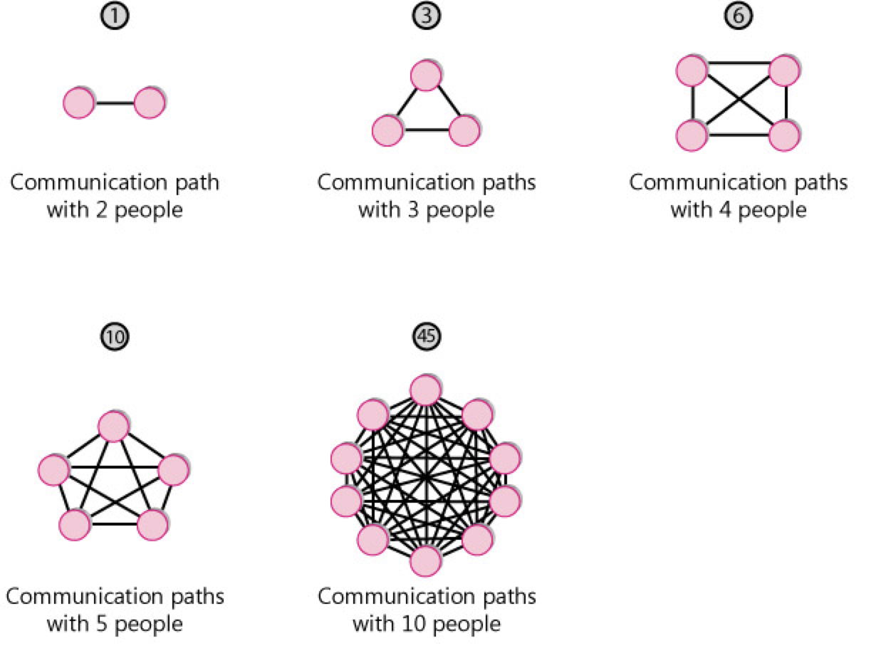
The consequence of this exponential increase in communication paths (along with some other factors) is that projects also have an exponential increase in effort as a project size increases. This is known as a diseconomy of scale.

Outside software, we usually discuss economies of scale rather than diseconomies of scale. An economy of scale is something like, "If we build a larger manufacturing plant, we'll be able to reduce the cost per unit we produce." An economy of scale implies that the bigger you get, the smaller the unit cost becomes.

A diseconomy of scale is the opposite. In software, the larger the system becomes, the greater the cost of each unit. If software exhibited economies of scale, a 100,000-LOC system would be less than 10 times as costly as a 10,000-LOC system. But the opposite is almost always the case.

---

# Count, Compute, Judge techniques

One of the secrets is that you should avoid doing what we traditionally think of as estimating! If you can count the answer directly, you should do that first. That approach produced the most accurate answer .

If you can't count the answer directly, you should count something else and then compute the answer by using some sort of calibration data.

Similarly, Lucy based her estimate on the documented fact of the room's occupancy limit. She used her judgment to estimate the room was 70 to 80 percent full.

---

# Delphi method

# Group Review

A simple technique for improving the accuracy of estimates created by individuals is to have a group review the estimates. When I have groups review estimates, I require three simple rules:

• Have each team member estimate pieces of the project individually, and then meet to compare your estimates Discuss differences in the estimates enough to understand the sources of the differences. Work until you reach consensus on high and low ends of estimation ranges.

• Don't just average your estimates and accept that You can compute the average, but you need to discuss the differences among individual results. Do not just take the calculated average automatically.

• Arrive at a consensus estimate that the whole group accepts If you reach an impasse, you can't vote. You must discuss differences and obtain buy-in from all group members.

The individual estimates average a Magnitude of Relative Error of 55%. The group-reviewed estimates average an error of only 30%. In this set of estimates, 92% of the group estimates were more accurate than the individual estimates and, on average, the reviews cut the error magnitude approximately in half.

# Wideband Delphi

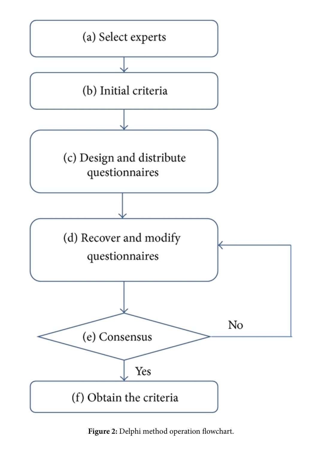
Wideband Delphi is a structured group-estimation technique. The original Delphi technique was developed by the Rand Corporation in the late 1940s for use in predicting trends in technology (Boehm 1981). The name Delphi comes from the ancient Greek oracle at Delphi. The basic Delphi technique called for several experts to create independent estimates and then to meet for as long as necessary to converge on, or at least agree upon, a single estimate.

Wideband Delphi Technique

1. The Delphi coordinator presents each estimator with the specification and an estimation form
2. Estimators prepare initial estimates individually. (Optionally, this step can be preformed after step 3.)
3. The coordinator calls a group meeting in which the estimators discuss estimation issues related to the project at hand. If the group agrees on a single estimate without much discussion, the coordinator assigns someone to play devil's advocate.
4. Estimators give their individual estimates to the coordinator anonymously.
5. The coordinator prepares a summary of the estimates on an iteration form and presents the iteration form to the estimators so that they can see how their estimates compare with other estimators' estimates.
6. The coordinator has estimators meet to discuss variations in their estimates.
7. Estimators vote anonymously on whether they want to accept the average estimate. If any of the estimators votes "no," they return to step 3.
8. The final estimate is the single-point estimate stemming from the Delphi exercise. Or, the final estimate is the range created through the Delphi discussion and the single-point Delphi estimate is the expected case.

---

# Challenges with Estimating Size

Numerous measures of size exist, including the following:

• Features
• User stories
• Story points
• Requirements
• Use cases
• Function points
• Web pages
• GUI components (windows, dialog boxes, reports, and so on)
• Database tables
• Interface definitions
• Classes
• Functions/subroutines
• Lines of code

The lines of code (LOC) measure is the most common size measure used for estimation, so we'll discuss that first.

Using lines of code is a mixed blessing for software estimation. On the positive side, lines of code present several advantages:

• Data on lines of code for past projects is easily collected via tools.
• Lots of historical data already exists in terms of lines of code in many organizations.
• Effort per line of code has been found to be roughly constant across programming languages, or close enough for practical purposes. (Effort per line of code is more a function of project size and kind of software than of programming language, as described in Chapter 5, "Estimate Influences." What you get for each line of code will vary dramatically, depending on the programming language.)
• Measurements in LOC allow for cross-project comparisons and estimation of future projects based on data from past projects.
• Most commercial estimation tools ultimately base their effort and schedule estimates on lines of code.

On the negative side, LOC measures present several difficulties when used to estimate size:

• Simple models such as "lines of code per staff month" are error-prone because of software's diseconomy of scale and because of vastly different coding rates for different kinds of software.
• LOC can't be used as a basis for estimating an individual's task assignments because of the vast differences in productivity between different programmers.
• A project that requires more code complexity than the projects used to calibrate the productivity assumptions can undermine an estimate's accuracy.
• Using the LOC measure as the basis for estimating requirements work, design work, and other activities that precede the creation of the code seems counterintuitive.
• Lines of code are difficult to estimate directly, and must be estimated by proxy.
• What exactly constitutes a line of code must be defined carefully to avoid the problems

---

# Challenges with Estimating Effort

Most projects eventually estimate effort directly from a detailed task list. But early in a project, effort estimates are most accurate when computed from size estimates. This chapter describes several means of computing those early estimates.

• Doing informal comparisons to past projects

• Computing Effort from Size

• Computing Effort Estimates by Using the Science of Estimation

  Use software tools based on the science of estimation to most accurately compute effort estimates from your size estimates

• Industry-Average Effort Graphs

  If you don't have your own historical data, you can look up a rough estimate of effort by using an effort graph

• ISBSG Method

  The International Software Benchmarking Standards Group (ISBSG) has developed an interesting and useful method of computing effort based on three factors: the size of a project in function points, the kind of development environment, and the maximum team size (ISBSG 2005). Presented by project type, the following eight equations are the ones you'd use to estimate effort using this approach. The equations produce an estimate in staff months, assuming 132 project-focused hours per staff month (that is, excluding vacations, holidays, training days, company meetings, and so on). The General formula is a general-purpose formula for use on all project types and is based on calibration data from about 600 projects. The other categories are calibrated with data from 63 to 363 projects.

---

# Challenges with Estimating Schedule

• Computing Schedule by Using Informal Comparisons to Past Projects
• Computing a Schedule Estimate by Using the Science of Estimation
• Schedule Compression and the Shortest Possible Schedule
  • Do not shorten a schedule estimate without increasing the effort estimate.
  • Do not shorten a nominal schedule more than 25%. In other words, keep your estimates out of the Impossible Zone.
  • Reduce costs by lengthening the schedule and conducting the project with a smaller team.
• Use schedule estimation to ensure your plans are plausible. Use detailed planning to produce the final schedule.
• Software tool calibrated with industry-average data
• Software tool calibrated with historical data

---

# Story based scope definition: scoping project, release planning

Making the Big Plan The purpose of the big plan is to answer the question "Should we invest more?" We address this question in three ways:

• Break the problem into pieces
• Bring the pieces into focus by estimating them
• Defer less valuable pieces

In release planning the customer chooses a few months' worth of stories, typically focusing on a public release.

The big plan helped us decide that it wasn't patently stupid to invest in the project. Now we need to synchronize the project with the business. We have to synchronize two aspects of the project:

• Date
• Scope

Even if the date of the next release is internally generated, it will be set for business reasons. You want to release often to stay ahead of your competition, but if you release too often, you won't ever have enough new functionality to merit a press release, a new round of sales calls, or champagne for the programmers.

Release planning allocates user stories to releases and iterations—what should we work on first? what will we work on later? The strategies you will use are similar to making the big plan in the first place:

• Break the big stories into smaller stories.
• Sharpen the focus on the stories by estimating how long each will take.
• Defer less valuable stories until what is left fits in the time available.

Release planning is a joint effort between the customer and the programmers. The customer drives release planning, and the programmers help navigate. The customer chooses which stories to place in the release and which stories to implement later, while the programmers provide the estimates required to make a sensible allocation.

The customer

• Defines the user stories
• Decides what business value the stories have
• Decides what stories to build in this release

The programmers

• Estimate how long it will take to build each story
• Warn the customer about significant technical risks
• Measure their team progress to provide the customer with an overall budget

---

Release Planning Events

• Changing the Priorities of Stories
• Adding a Story
• Rebuild the Release Plan

---

The First Plan

• Making the First Plan
• Choosing Your Iteration Length

---

Release Planning Variations

• Short Releases
• Long Releases
• Small Stories

---

# Documenting and presenting estimation results

An essential practice in presenting an estimate is to document the assumptions embodied in the estimate. Assumptions fall into several familiar categories:

• Which features are required
• Which features are not required
• How elaborate certain features need to be
• Availability of key resources
• Dependencies on third-party performance
• Major unknowns
• Major influences and sensitivities of the estimate
• How good the estimate is
• What the estimate can be used for

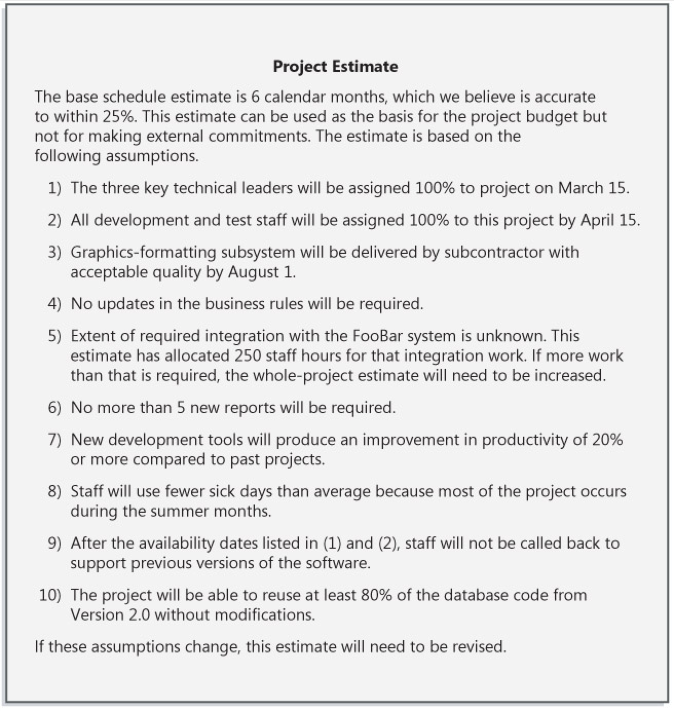
example of an estimate that's presented with documented assumptions. By documenting and communicating your assumptions, you help to set the expectation that your software project is subject to variability.

---

# PERT analysis

PERT предназначен для очень масштабных, единовременных, сложных, нерутинных проектов. Метод подразумевает наличие неопределённости, давая возможность разработать рабочий график проекта без точного знания деталей и необходимого времени для всех его составляющих.

PERT был разработан главным образом для упрощения планирования на бумаге и составления графиков больших и сложных проектов. Метод в особенности нацелен на анализ времени, которое требуется для выполнения каждой отдельной задачи, а также определение минимального необходимого времени для выполнения всего проекта.

Самой популярной частью PERT является метод критического пути, опирающийся на построение сетевого графика (сетевой диаграммы PERT).

• Событие PERT (PERT event) — момент, отмечающий начало или окончание одной или нескольких задач. Событие не имеет длительности и не потребляет ресурсы. В случае, если событие отмечает завершение нескольких задач, оно не «наступает» (не происходит) до того, пока все задачи, приводящие к событию, не будут выполнены.

• *Предшествующее событие(predecessor event) — событие, которое предшествует некоторому другому событию непосредственно, без промежуточных событий. Любое событие может иметь несколько предшествующих событий и может быть предшественником для нескольких событий.

• Последующее событие(successor event) — событие, которое следует за некоторым событием непосредственно, без промежуточных событий. Любое событие может иметь несколько последующих событий и может быть последователем нескольких событий.

• Задача PERT(PERT activity) — конкретная работа (задача), которое имеет длительность и требует ресурсов для выполнения. Примерами ресурсов являются исполнители, сырьё, пространство, оборудование, техника и т. д. Невозможно начать выполнение задачи PERT, пока не наступили все предшествующие ей события.

• Оптимистическое время (optimistic time) t_o — минимальное возможная длительность выполнения задачи в предположении, что всё происходит наилучшим или наиболее удачным образом.

• Пессимистическое время(pessimistic time) t_p — максимально возможная длительность выполнения задачи в предположении, что всё происходит наихудшим или наименее удачным образом (исключая крупные катастрофы).

• Наиболее вероятное время(most likely time) t_m — длительность выполнения задачи в предположении, что всё происходит так, как бывает чаще всего (как обычно).

• Ожидаемое время(expected time) t_e — оценка длительности выполнения задачи на основе оценок оптимистического, пессимистического и наиболее вероятного времени:

• Проскальзывание или провисание(float, slack) — мера дополнительного времени и ресурсов, доступных для выполнения работы. Время, на которое выполнение задачи может быть сдвинуто без задержки любых последующих задач (свободное проскальзывание) или всего проекта (общее проскальзывание). Позитивное провисание показывает опережение расписания, негативное провисание показывает отставание, и нулевое провисание показывает соответствие расписанию.

• Критический путь(critical path) — длиннейший маршрут на пути от начального до финального события. Критический путь определяет минимальное время, требуемое для выполнения всего проекта, и, таким образом, любые задержки на критическом пути соответственно задерживают достижение финального события.

• Критическая задача(critical activity) — задача, проскальзывание которой равно нулю. Задача с нулевым проскальзыванием не обязательно должна находиться на критическом пути, но все задачи на критических путях имеют нулевое проскальзывание.

• Быстрый проход(fast tracking) — метод уменьшения общей длительности проекта путём параллельного выполнения задач, которые в обычной ситуации выполнялись бы последовательно, например, проектирование и строительство.

---

Пример сетевой диаграммы PERT для проекта продолжительностью в семь месяцев с пятью промежуточными точками (от 10 до 50) и шестью деятельностями (от A до F).

Самая известная часть PERT — это диаграммы взаимосвязей работ и событий. Предлагает использовать диаграммы-графы с работами на узлах, с работами на стрелках (сетевые графики), а так же диаграммы Ганта.

Диаграмма PERT с работами на стрелках представляет собой множество точек-вершин (события) вместе с соединяющими их ориентированными дугами (работы). Всякой дуге, рассматриваемой в качестве какой-то работы из числа нужных для осуществления проекта, приписываются определенные количественные характеристики. Это — объемы выделяемых на данную работу ресурсов и, соответственно, ее ожидаемая продолжительность (длина дуги). Любая вершина интерпретируется как событие завершения работ, представленных дугами, которые входят в нее, и одновременно начала работ, отображаемых дугами, исходящими оттуда. Таким образом, отражается тот факт, что ни к одной из работ нельзя приступить прежде, чем будут выполнены все работы, предшествующие ей согласно технологии реализации проекта. Начало этого процесса — вершина без входящих, а окончание — вершина без исходящих дуг. Остальные вершины должны иметь и те, и другие дуги.

Последовательность дуг, в которой конец каждой предшествующей совпадает с началом последующей, трактуется как путь от отправной вершины к завершающей, а сумма длин таких дуг — как его продолжительность. Обычно начало и конец реализации проекта связаны множеством путей, длины которых различаются. Наибольшая определяет длительность всего этого проекта, минимально возможную при зафиксированных характеристиках дуг графа. Соответствующий путь — критический, то есть именно от продолжительности составляющих его работ зависит общая продолжительность проекта, хотя при изменении продолжительности любых работ проекта критическим может стать и другой путь.